(Step 3) Model Construction¶

Always find the best classification technique¶

Shihab [Shi12] and Hall et al. [HBB+12] show that logistic regression and random forests are the two most-popularly-used classification techniques in the literature of software defect prediction, since they are explainable and have built-in model explanation techniques (i.e., the ANOVA analysis for the regression technique and the variable importance analysis for the random forests technique). Recent studies [TMHM16a][FMS16][TMHM18] also demonstrate that automated parameter optimisation can improve the performance and stability of defect models. Using the findings of prior studies to guide our selection, we choose (1) the commonly-used classification techniques that have built-in model-specific explanation techniques (i.e., logistic regression and random forests) and (2) the top-5 classification techniques when performing automated parameter optimisation [TMHM16a][TMHM18] (i.e., random forests, C5.0, neural network, GBM, and xGBTree).

To determine the best classification technique, we use the Area Under the receiver operator characteristic Curve (AUC) to as a performance indicator to measure the discriminatory power of predictive models, as suggested by recent research [LBMP08][GMH15][RD13]. The axes of the curve of the AUC measure are the coverage of non-defective modules (true negative rate) for the x-axis and the coverage of defective modules (true positive rate) for the y-axis. The AUC measure is a threshold-independent performance measure that evaluates the ability of models in discriminating between defective and clean instances. The values of AUC range between 0 (worst), 0.5 (no better than random guessing), and 1 (best) [HM82]. We neither re-balance nor normalize our training samples to preserve its original characteristics and to avoid any concept drift for the explanations of defect models[THM19].

Below, we provide an example of an interactive code snippet on how to construct and evaluate defect models to find the best classification techniques.

# Import for Construct Defect Models (Classification)
from sklearn.linear_model import LogisticRegression # Logistic Regression
from sklearn.ensemble import RandomForestClassifier # Random Forests
from sklearn.tree import DecisionTreeClassifier # C5.0 (Decision Tree)
from sklearn.neural_network import MLPClassifier # Neural Network
from sklearn.ensemble import GradientBoostingClassifier # Gradient Boosting Machine (GBM)
import xgboost as xgb # eXtreme Gradient Boosting Tree (xGBTree)

# Import for AUC calculation
from sklearn.metrics import roc_auc_score 

## Construct defect models

# Logistic Regression
lr_model = LogisticRegression(random_state=1234)
lr_model.fit(X_train, y_train)  
lr_model_AUC = round(roc_auc_score(y_test, lr_model.predict_proba(X_test)[:,1]), 3)

# Random Forests
rf_model = RandomForestClassifier(random_state=1234, n_jobs = 10)
rf_model.fit(X_train, y_train)  
rf_model_AUC = round(roc_auc_score(y_test, rf_model.predict_proba(X_test)[:,1]), 3)

# C5.0 (Decision Tree)
dt_model = DecisionTreeClassifier(random_state=1234)
dt_model.fit(X_train, y_train)  
dt_model_AUC = round(roc_auc_score(y_test, dt_model.predict_proba(X_test)[:,1]), 3)

# Neural Network
nn_model = MLPClassifier(random_state=1234)
nn_model.fit(X_train, y_train)  
nn_model_AUC = round(roc_auc_score(y_test, nn_model.predict_proba(X_test)[:,1]), 3)

# Gradient Boosting Machine (GBM)
gbm_model = GradientBoostingClassifier(random_state=1234)
gbm_model.fit(X_train, y_train)  
gbm_model_AUC = round(roc_auc_score(y_test, gbm_model.predict_proba(X_test)[:,1]), 3)

# eXtreme Gradient Boosting Tree (xGBTree)
xgb_model = xgb.XGBClassifier(random_state=1234)
xgb_model.fit(X_train, y_train)  
xgb_model_AUC = round(roc_auc_score(y_test, xgb_model.predict_proba(X_test)[:,1]), 3)

# Summarise into a DataFrame
model_performance_df = pd.DataFrame(data=np.array([['Logistic Regression', 'Random Forests', 'C5.0 (Decision Tree)', 'Neural Network', 'Gradient Boosting Machine (GBM)', 'eXtreme Gradient Boosting Tree (xGBTree)'],
                            [lr_model_AUC, rf_model_AUC, dt_model_AUC, nn_model_AUC, gbm_model_AUC, xgb_model_AUC]]).transpose(),
             index = range(6),
             columns = ['Model', 'AUC'])
model_performance_df['AUC'] = model_performance_df.AUC.astype(float)
model_performance_df = model_performance_df.sort_values(by = ['AUC'], ascending = False)

# Visualise the performance of defect models
display(model_performance_df)
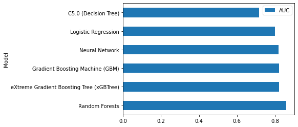
model_performance_df.plot(kind = 'barh', y = 'AUC', x = 'Model')

	Model	AUC
1	Random Forests	0.859
5	eXtreme Gradient Boosting Tree (xGBTree)	0.822
4	Gradient Boosting Machine (GBM)	0.821
3	Neural Network	0.819
0	Logistic Regression	0.799
2	C5.0 (Decision Tree)	0.717

<AxesSubplot:ylabel='Model'>

Note

Parts of this chapter have been published by Jirayus Jiarpakdee, Chakkrit Tantithamthavorn, Hoa K. Dam, John Grundy: An Empirical Study of Model-Agnostic Techniques for Defect Prediction Models. IEEE Trans. Software Eng. (2021).

Explainable AI for Software Engineering

(Step 3) Model Construction¶

Always find the best classification technique¶

Suggested Readings¶